

How Many Discrete Band Pass Filters Does The 7300 Include?
8. Filters
In this chapter nosotros acquire virtually digital filters using Python. We cover types of filters (FIR/IIR and low-laissez passer/high-pass/band-laissez passer/ring-stop), how filters are represented digitally, and how they are designed. We finish with an introduction to pulse shaping, which we further explore in the Pulse Shaping chapter.
Filter Basics
Filters are used in many disciplines. For example, image processing makes heavy use of second filters, where the input and output are images. Yous might use a filter every morning to brand your java, which filters out solids from liquid. In DSP, filters are primarily used for:
- Separation of signals that take been combined (e.g., extracting the point you desire)
- Removal of excess noise later receiving a betoken
- Restoration of signals that accept been distorted in some manner (east.g., an sound blaster is a filter)
At that place are certainly other uses for filters, merely this affiliate is meant to introduce the concept rather than explain all the ways filtering can happen.
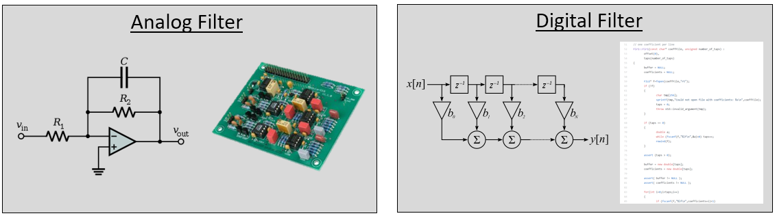
Y'all may think we only care well-nigh digital filters; this textbook explores DSP, after all. However, it's important to know that a lot of filters will exist analog, like those in our SDRs placed before the analog-to-digital converter (ADC) on the receive side. The post-obit paradigm juxtaposes a schematic of an analog filter circuit with a flowchart representation of a digital filtering algorithm.
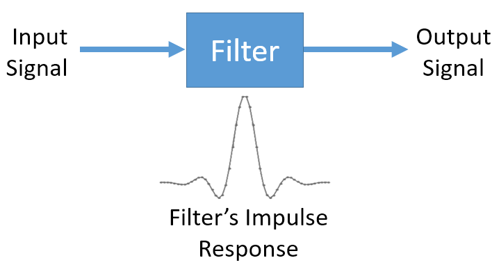
In DSP, where the input and output are signals, a filter has one input signal and one output signal:

You cannot feed two dissimilar signals into a single filter without adding them together first or doing some other operation. Too, the output will ever exist one indicate, i.due east., a 1D array of numbers.
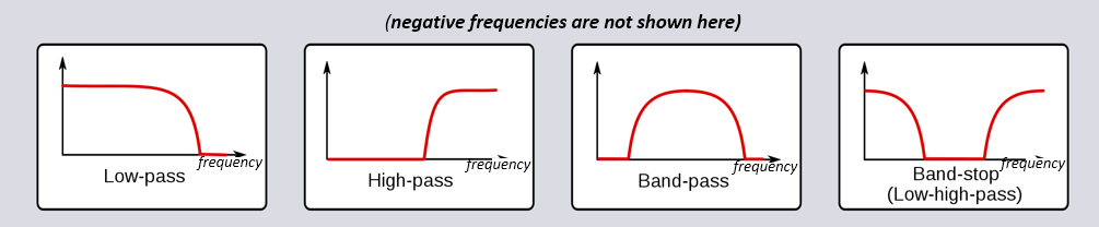
There are four bones types of filters: low-pass, high-pass, ring-laissez passer, and band-stop. Each type modifies signals to focus on unlike ranges of frequencies within them. The graphs below demonstrate how frequencies in signals are filtered for each blazon.
(Add together DIAGRAM SHOWING NEGATIVE FREQS Likewise)
Each filter permits certain frequencies to remain from a signal while blocking other frequencies. The range of frequencies a filter lets through is known every bit the "passband", and "stopband" refers to what is blocked. In the case of the low-laissez passer filter, it passes low frequencies and stops high frequencies, and so 0 Hz will e'er be in the passband. For a loftier-pass and band-laissez passer filter, 0 Hz will ever be in the stopband.
Practise non misfile these filtering types with filter algorithmic implementation (e.grand., IIR vs FIR). The most common type by far is the low-pass filter (LPF) considering we often stand for signals at baseband. LPF allows us to filter out everything "around" our point, removing backlog noise and other signals.
Filter Representation
For about filters nosotros will run across (known equally FIR, or Finite Impulse Response, type filters), we can represent the filter itself with a single array of floats. For filters symmetrical in the frequency domain, these floats will be real (versus complex), and at that place tends to be an odd number of them. We call this array of floats "filter taps". Nosotros often use  every bit the symbol for filter taps. Here is an example of a set of filter taps, which ascertain i filter:
h = [ 9.92977939e-04 1.08410297e-03 8.51595307e-04 1.64604862e-04 - 1.01714338e-03 - ii.46268845e-03 - 3.58236429e-03 - iii.55412543e-03 - one.68583512e-03 two.10562324e-03 6.93100252e-03 1.09302641e-02 1.17766532e-02 7.60955496e-03 - 1.90555639e-03 - ane.48306750e-02 - 2.69313236e-02 - 3.25659606e-02 - 2.63400086e-02 - 5.04184562e-03 3.08099470e-02 vii.64264738e-02 one.23536693e-01 1.62377258e-01 one.84320776e-01 1.84320776e-01 1.62377258e-01 1.23536693e-01 7.64264738e-02 three.08099470e-02 - 5.04184562e-03 - two.63400086e-02 - three.25659606e-02 - 2.69313236e-02 - 1.48306750e-02 - 1.90555639e-03 seven.60955496e-03 i.17766532e-02 ane.09302641e-02 six.93100252e-03 2.10562324e-03 - one.68583512e-03 - 3.55412543e-03 - 3.58236429e-03 - 2.46268845e-03 - i.01714338e-03 i.64604862e-04 8.51595307e-04 i.08410297e-03 9.92977939e-04 ] Instance Utilize-Instance
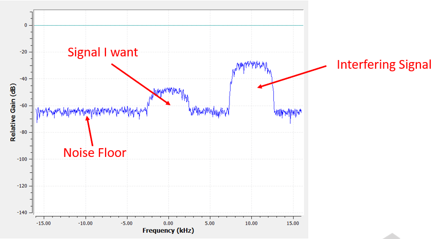
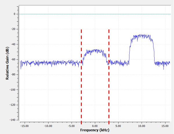
To larn how filters are used, let'south look an an example where we melody our SDR to a frequency of an existing bespeak, and nosotros want to isolate it from other signals. Remember that we tell our SDR which frequency to tune to, but the samples that the SDR captures are at baseband, meaning the signal volition display every bit centered around 0 Hz. We volition have to keep track of which frequency we told the SDR to tune to. Here is what nosotros might receive:
Considering our bespeak is already centered at DC (0 Hz), we know we want a low-pass filter. We must choose a "cutoff frequency" (a.1000.a. corner frequency), which will determine when the passband transitions to stopband. Cutoff frequency will always be in units of Hz. In this example, 3 kHz seems similar a good value:
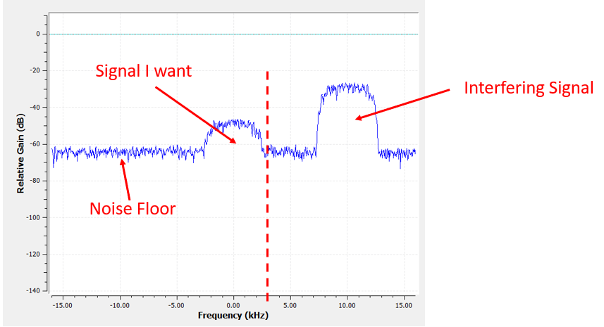
However, the way most depression-laissez passer filters work, the negative frequency boundary will be -iii kHz besides. I.e., it'south symmetrical around DC (afterward on you will see why). Our cutoff frequencies will expect something like this (the passband is the area in between):
After creating and applying the filter with a cutoff freq of 3 kHz, we now accept:
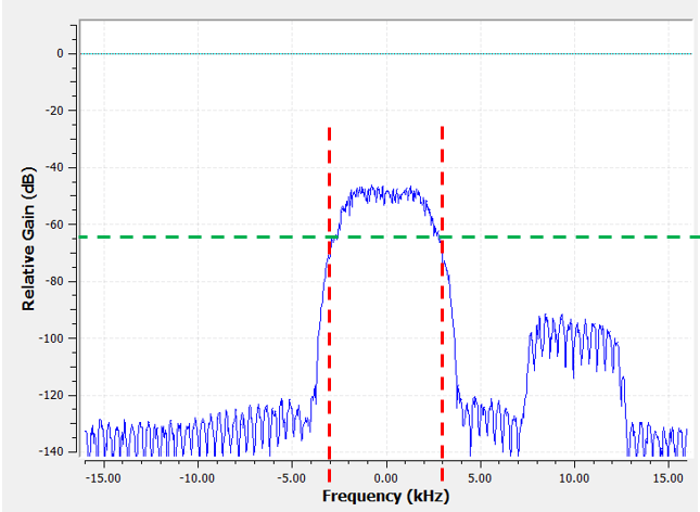
This filtered signal will look confusing until you lot recall that our noise floor was at the green line around -65 dB. Even though we can still see the interfering signal centered at 10 kHz, we have severely decreased the power of that signal. Information technology'southward now below where the noise floor was! We besides removed near of the noise that existed in the stopband.
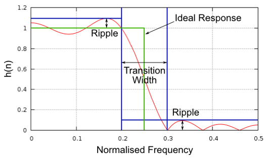
In addition to cutoff frequency, the other main parameter of our low-pass filter is chosen the "transition width". Transition width, also measured in Hz, instructs the filter how quickly it has to go between the passband and stopband since an instant transition is impossible.
Let's visualize transition width. In the diagram below, the green line represents the ideal response for transitioning between a passband and stopband, which essentially has a transition width of nil. The Red line demonstrates the effect of a realistic filter, which has some ripple and a certain transition width.
You might be wondering why nosotros wouldn't simply set up the transition width as small equally possible. The reason is mainly that a smaller transition width results in more than taps, and more than taps ways more than computations–we volition see why shortly. A 50-tap filter can run all solar day long using i% of the CPU on a Raspberry Pi. Meanwhile, a fifty,000 tap filter will cause your CPU to explode! Typically we employ a filter designer tool, then run across how many taps it outputs, and if it's way too many (e.g., more than 100) we increase the transition width. It all depends on the application and hardware running the filter, of course.
In the filtering case above, nosotros had used a cutoff of 3 kHz and a transition width of 1 kHz (information technology's hard to really see the transition width merely looking at these screenshots). The resulting filter had 77 taps.
Back to filter representation. Even though nosotros might show the listing of taps for a filter, we ordinarily represent filters visually in the frequency domain. We telephone call this the "frequency response" of the filter, and it shows the states the beliefs of the filter in frequency. Here is the frequency response of the filter we were just using:
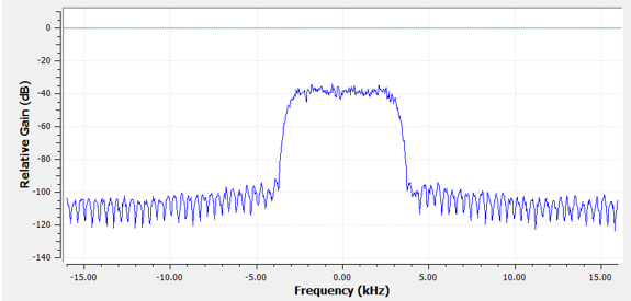
Note that what I'grand showing here is not a point–it'southward but the frequency domain representation of the filter. That can exist a picayune hard to wrap your head around at start, simply as we expect at examples and code, it volition click.
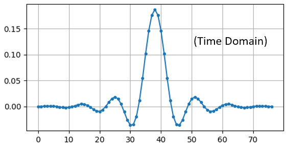
A given filter also has a time domain representation; it's called the "impulse response" of the filter because it is what you lot see in the fourth dimension domain if y'all take an impulse and put it through the filter. (Google "Dirac delta function" for more than info near what an impulse is). For a FIR type filter, the impulse response is simply the taps themselves. For that 77 tap filter we used earlier, the taps are:
h = [ - 0.00025604525581002235 , 0.00013669139298144728 , 0.0005385575350373983 , 0.0008378280326724052 , 0.000906112720258534 , 0.0006353431381285191 , - nine.884083502996931e-19 , - 0.0008822851814329624 , - 0.0017323142383247614 , - 0.0021665366366505623 , - 0.0018335371278226376 , - 0.0005912294145673513 , 0.001349081052467227 , 0.0033936649560928345 , 0.004703888203948736 , 0.004488115198910236 , 0.0023609865456819534 , - 0.0013707970501855016 , - 0.00564080523326993 , - 0.008859002031385899 , - 0.009428252466022968 , - 0.006394983734935522 , 4.76480351940553e-18 , 0.008114570751786232 , 0.015200719237327576 , 0.018197273835539818 , 0.01482443418353796 , 0.004636279307305813 , - 0.010356673039495945 , - 0.025791890919208527 , - 0.03587324544787407 , - 0.034922562539577484 , - 0.019146423786878586 , 0.011919975280761719 , 0.05478153005242348 , 0.10243935883045197 , 0.1458890736103058 , 0.1762896478176117 , 0.18720689415931702 , 0.1762896478176117 , 0.1458890736103058 , 0.10243935883045197 , 0.05478153005242348 , 0.011919975280761719 , - 0.019146423786878586 , - 0.034922562539577484 , - 0.03587324544787407 , - 0.025791890919208527 , - 0.010356673039495945 , 0.004636279307305813 , 0.01482443418353796 , 0.018197273835539818 , 0.015200719237327576 , 0.008114570751786232 , 4.76480351940553e-eighteen , - 0.006394983734935522 , - 0.009428252466022968 , - 0.008859002031385899 , - 0.00564080523326993 , - 0.0013707970501855016 , 0.0023609865456819534 , 0.004488115198910236 , 0.004703888203948736 , 0.0033936649560928345 , 0.001349081052467227 , - 0.0005912294145673513 , - 0.0018335371278226376 , - 0.0021665366366505623 , - 0.0017323142383247614 , - 0.0008822851814329624 , - 9.884083502996931e-19 , 0.0006353431381285191 , 0.000906112720258534 , 0.0008378280326724052 , 0.0005385575350373983 , 0.00013669139298144728 , - 0.00025604525581002235 ] And even though we haven't gotten into filter blueprint yet, here is the Python code that generated that filter:
import numpy equally np from scipy import signal import matplotlib.pyplot equally plt num_taps = 51 # it helps to employ an odd number of taps cut_off = 3000 # Hz sample_rate = 32000 # Hz # create our low pass filter h = signal . firwin ( num_taps , cut_off , nyq = sample_rate / 2 ) # plot the impulse response plt . plot ( h , '.-' ) plt . show () But plotting this assortment of floats gives us the filter'south impulse response:
And here is the code that was used to produce the frequency response, shown earlier. Information technology's a little more complicated because we have to create the x-axis array of frequencies.
# plot the frequency response H = np . abs ( np . fft . fft ( h , 1024 )) # take the 1024-signal FFT and magnitude H = np . fft . fftshift ( H ) # brand 0 Hz in the heart due west = np . linspace ( - sample_rate / two , sample_rate / 2 , len ( H )) # x axis plt . plot ( w , H , '.-' ) plt . prove () Real vs. Complex Filters
The filter I showed you lot had real taps, but taps tin can also exist complex. Whether the taps are real or complex doesn't take to match the point you put through information technology, i.e., you lot can put a circuitous betoken through a filter with existent taps and vice versa. When the taps are real, the filter's frequency response will be symmetrical around DC (0 Hz). Typically we employ complex taps when we need disproportion, which does not happen too oftentimes.

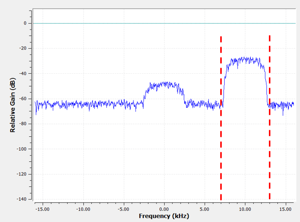
As an example of complex taps, let'due south go back to the filtering use-case, except this fourth dimension we want to receive the other interfering signal (without having to re-melody the radio). That means we want a band-laissez passer filter, but not a symmetrical one. We just want to go on (a.1000.a "pass") frequencies between around 7 kHz to thirteen kHz (we don't want to also laissez passer -xiii kHz to -vii kHz):
1 way to design this kind of filter is to brand a low-pass filter with a cutoff of 3 kHz and and so frequency shift information technology. Remember that we can frequency shift 10(t) (time domain) by multiplying it past  . In this case
  should exist 10 kHz, which shifts our filter up by 10 kHz. Recollect that in our Python code from to a higher place, was the filter taps of the low-pass filter. In social club to create our band-pass filter we just take to multiply those taps by , although it involves creating a vector to represent time based on our sample period (inverse of the sample rate):
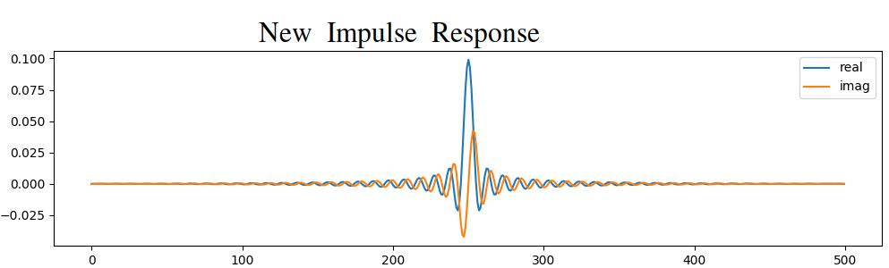
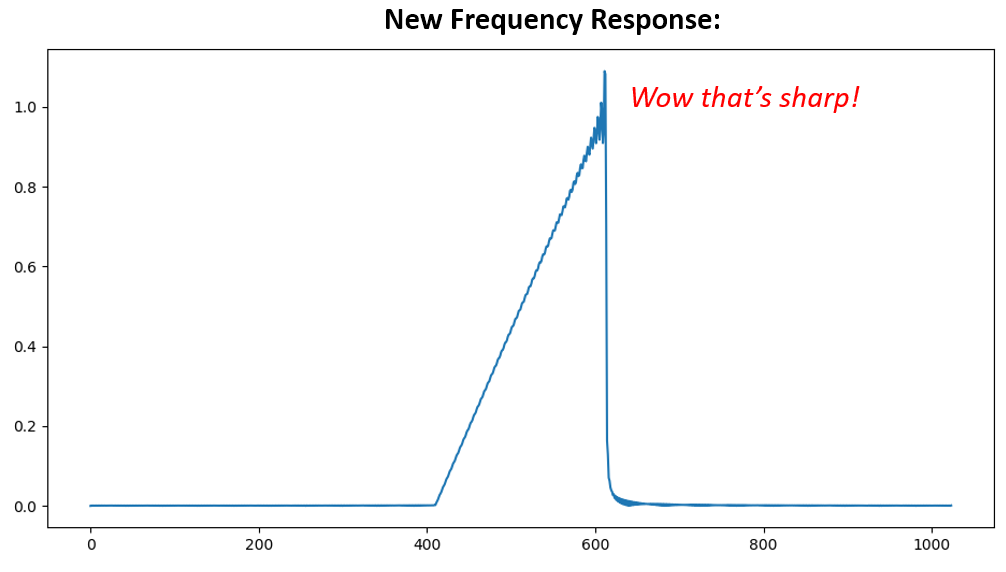
# (h was constitute using the beginning code snippet) # Shift the filter in frequency by multiplying past exp(j*2*pi*f0*t) f0 = 10e3 # amount we will shift Ts = 1.0 / sample_rate # sample period t = np . arange ( 0.0 , Ts * len ( h ), Ts ) # time vector. args are (showtime, finish, step) exponential = np . exp ( 2 j * np . pi * f0 * t ) # this is essentially a complex sine wave h_band_pass = h * exponential # practice the shift # plot impulse response plt . figure ( 'impulse' ) plt . plot ( np . real ( h_band_pass ), '.-' ) plt . plot ( np . imag ( h_band_pass ), '.-' ) plt . legend ([ 'existent' , 'imag' ], loc = 1 ) # plot the frequency response H = np . abs ( np . fft . fft ( h_band_pass , 1024 )) # take the 1024-bespeak FFT and magnitude H = np . fft . fftshift ( H ) # brand 0 Hz in the middle w = np . linspace ( - sample_rate / 2 , sample_rate / 2 , len ( H )) # x axis plt . figure ( 'freq' ) plt . plot ( w , H , '.-' ) plt . xlabel ( 'Frequency [Hz]' ) plt . testify () The plots of the impulse response and frequency response are shown below:
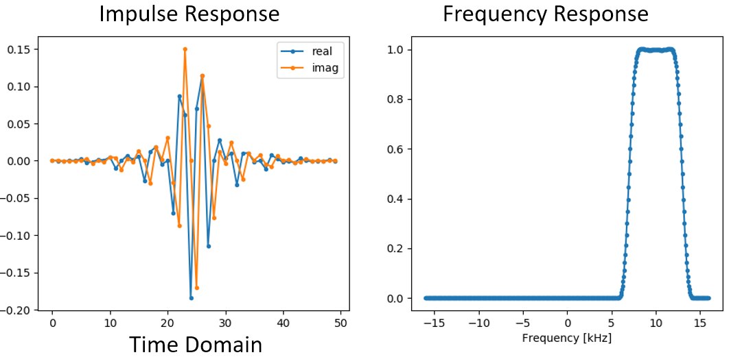
Considering our filter is not symmetrical around 0 Hz, it has to apply complex taps. Therefore we demand 2 lines to plot those circuitous taps. What we see in the left-paw plot above is still the impulse response. Our frequency response plot is what really validates that we created the kind of filter we were hoping for, where it will filter out everything except the point centered effectually 10 kHz. Once again, recollect that the plot above is not an actual signal: information technology's just a representation of the filter. Information technology tin be very confusing to grasp because when you utilize the filter to the bespeak and plot the output in the frequency domain, in many cases it will look roughly the same equally the filter'due south frequency response itself.
If this subsection added to the confusion, don't worry, 99% of the time you lot'll be dealing with unproblematic low pass filters with real taps anyhow.
Filter Implementation
We aren't going to dive also securely into the implementation of filters. Rather, I focus on filter design (you can observe prepare-to-utilize implementations in any programming language anyway). For now, here is 1 take-abroad: to filter a signal with an FIR filter, you simply convolve the impulse response (the array of taps) with the input signal. (Don't worry, a later section explains convolution.) In the discrete world we employ a discrete convolution (instance below). The triangles labeled as b's are the taps. In the flowchart, the squares labeled  higher up the triangles signify to delay by 1 time footstep.
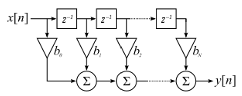
You might be able to encounter why we call them filter "taps" at present, based on the way the filter itself is implemented.
FIR vs IIR
There are 2 chief classes of digital filters: FIR and IIR
- Finite impulse response (FIR)
- Infinite impulse response (IIR)
Nosotros won't get also deep into the theory, merely for now but remember: FIR filters are easier to design and can do anything you want if you use enough taps. IIR filters are more complicated with the potential to be unstable, just they are more efficient (use less CPU and memory for the given filter). If someone merely gives you a list of taps, information technology'due south assumed they are taps for an FIR filter. If they beginning mentioning "poles", they are talking about IIR filters. We will stick with FIR filters in this textbook.
Below is an case frequency response, comparison an FIR and IIR filter that do nearly exactly the same filtering; they accept a like transition-width, which every bit we learned volition determine how many taps are required. The FIR filter has 50 taps and the IIR filter has 12 poles, which is similar having 12 taps in terms of computations required.
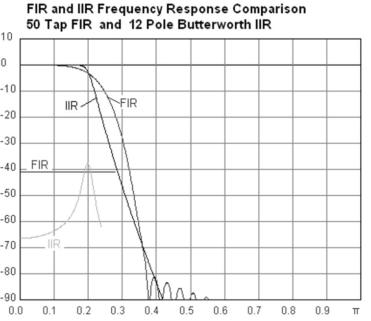
The lesson is that the FIR filter requires vastly more computational resources than the IIR to perform roughly the same filtering operation.
Here are some real-world examples of FIR and IIR filters that you may have used before.
If you perform a "moving average" across a list of numbers, that'southward just an FIR filter with taps of ane's: - h = [one i 1 ane ane ane 1 1 1 1] for a moving boilerplate filter with a window size of 10. It also happens to exist a low-pass type filter; why is that? What'south the difference betwixt using one's and using taps that decay to zero?
Answers
A moving boilerplate filter is a low-pass filter because it smooths out "loftier frequency" changes, which is usually why people volition use one. The reason to apply taps that decay to nix on both ends is to avoid a sudden alter in the output, like if the point being filtered was zero for a while and and so suddenly jumped up.
Now for an IIR example. Have any of you always done this:
x = x*0.99 + new_value*0.01
where the 0.99 and 0.01 stand for the speed the value updates (or rate of disuse, same thing). It's a convenient manner to slowly update some variable without having to remember the last several values. This is really a course of depression-pass IIR Filter. Hopefully you can see why IIR filters have less stability than FIR. Values never fully go away!
Convolution
We volition take a brief detour to introduce the convolution operator. Feel costless to skip this section if you lot are already familiar with information technology.
Calculation two signals together is one way of combining two signals into one. In the Frequency Domain chapter we explored how the linearity property applies when adding two signals together. Convolution is another mode to combine ii signals into i, but information technology is very dissimilar than only calculation them. The convolution of 2 signals is like sliding ane across the other and integrating. It is very like to a cantankerous-correlation, if you are familiar with that functioning. In fact it is equivalent to a cross-correlation in many cases.
I believe the convolution operation is best learned through examples. In this offset example, we convolve two foursquare pulses together:

Because information technology's just a sliding integration, the result is a triangle with a maximum at the point where both square pulses lined upwards perfectly. Allow's look at what happens if we convolve a square pulse with a triangular pulse:

In both examples, we have two input signals (1 carmine, i blue), and then the output of the convolution is displayed. You can see that the output is the integration of the two signals as ane slides across the other. Because of this "sliding" nature, the length of the output is actually longer than the input. If 1 signal is Grand samples and the other signal is N samples, the convolution of the 2 tin can produce N+One thousand-1 samples. However, functions such every bit numpy.convolve() accept a mode to specify whether you want the whole output ( max(M, N) samples) or simply the samples where the signals overlapped completely ( max(M, N) - min(M, North) + i if you were curious). No demand to get caught up in this detail. Just know that the length of the output of a convolution is not just the length of the inputs.
So why does convolution matter in DSP? Well for starters, to filter a signal, we can just take the impulse response of that filter and convolve it with the signal. FIR filtering is but a convolution performance.
It might be confusing because before we mentioned that convolution takes in two signals and outputs 1. We can care for the impulse response like a betoken, and convolution is a math operator after all, which operates on ii 1D arrays. If one of those 1D arrays is the filter's impulse response, the other 1D assortment tin be a slice of the input signal, and the output will be a filtered version of the input.
Let'southward meet some other example to help this click. In the example below, the triangle will represent our filter'south impulse response, and the green point is our signal being filtered.
The red output is the filtered bespeak.
Question: What type of filter was the triangle?
Answers
It smoothed out the high frequency components of the light-green signal (i.east., the sharp transitions of the square) so it acts as a low-laissez passer filter.
Now that we are starting to empathise convolution, I will present the mathematical equation for information technology. The asterisk (*) is typically used as the symbol for convolution:

In this above expression,  is the point or input that is flipped and slides across
  , but and can be swapped and information technology's still the same expression. Typically, the shorter array volition be used as . Convolution is equal to a cross-correlation, defined as
  , when is symmetrical, i.eastward., it doesn't change when flipped about the origin.
Filter Design in Python
At present nosotros will consider i way to design an FIR filter ourselves in Python. While at that place are many approaches to designing filters, we will utilise the method of starting in the frequency domain and working backwards to find the impulse response. Ultimately that is how our filter is represented (by its taps).
You offset by creating a vector of your desired frequency response. Let's design an arbitrarily shaped depression-pass filter shown below:
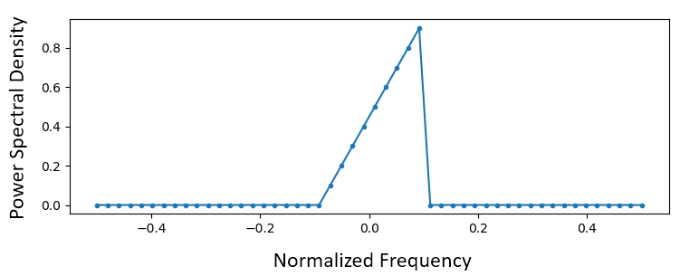
The code used to create this filter is fairly uncomplicated:
import numpy as np import matplotlib.pyplot every bit plt H = np . hstack (( np . zeros ( 20 ), np . arange ( 10 ) / 10 , np . zeros ( 20 ))) w = np . linspace ( - 0.5 , 0.5 , 50 ) plt . plot ( west , H , '.-' ) plt . show () hstack() is ane fashion to concatenate arrays in numpy. We know it will lead to a filter with complex taps. Why?
Respond
It'southward not symmetrical around 0 Hz.
Our end goal is to find the taps of this filter so we can actually use it. How practise nosotros get the taps, given the frequency response? Well, how practice we catechumen from the frequency domain back to the fourth dimension domain? Changed FFT (IFFT)! Recall that the IFFT function is almost exactly the aforementioned as the FFT function. We likewise need to IFFTshift our desired frequency response before the IFFT, and and then nosotros need yet another IFFshift after the IFFT (no, they don't abolish themselves out, you can try). This procedure might seem confusing. But call up that you always should FFTshift after an FFT and IFFshift after an IFFT.
h = np . fft . ifftshift ( np . fft . ifft ( np . fft . ifftshift ( H ))) plt . plot ( np . existent ( h )) plt . plot ( np . imag ( h )) plt . legend ([ 'real' , 'imag' ], loc = i ) plt . show () 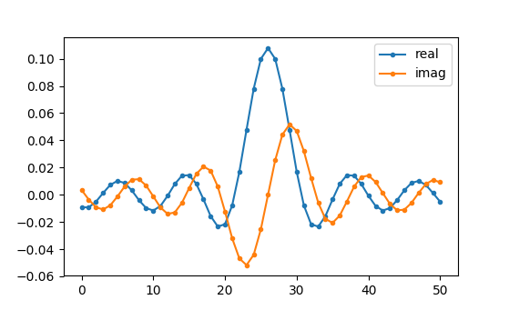
We will use these taps shown above as our filter. Nosotros know that the impulse response is plotting the taps, so what we see in a higher place is our impulse response. Let'southward take the FFT of our taps to encounter what the frequency domain actually looks like. We will do a one,024 point FFT to get a high resolution:
H_fft = np . fft . fftshift ( np . abs ( np . fft . fft ( h , 1024 ))) plt . plot ( H_fft ) plt . show () 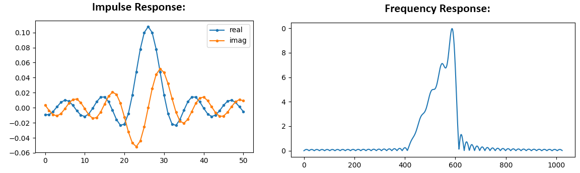
See how the frequency response non very straight… it doesn't match our original very well, if you recall the shape that we initially wanted to brand a filter for. A big reason is because our impulse response isn't done decaying, i.eastward., the left and right sides don't reach zero. We take two options that will permit information technology to disuse to zero:
Option 1: We "window" our current impulse response so that information technology decays to 0 on both sides. It involves multiplying our impulse response with a "windowing function" that starts and ends at nil.
# After creating h using the previous lawmaking, create and utilize the window window = np . hamming ( len ( h )) h = h * window 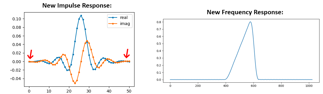
Option two: Nosotros re-generate our impulse response using more than points so that it has time to decay. Nosotros demand to add resolution to our original frequency domain assortment (called interpolating).
H = np . hstack (( np . zeros ( 200 ), np . arange ( 100 ) / 100 , np . zeros ( 200 ))) w = np . linspace ( - 0.5 , 0.5 , 500 ) plt . plot ( w , H , '.-' ) plt . show () # (the rest of the code is the same) 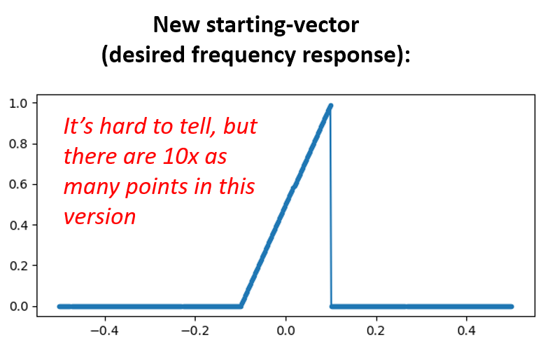
Both options worked. Which ane would you choose? The second method resulted in more than taps, but the first method resulted in a frequency response that wasn't very sharp and had a falling border wasn't very steep. There are numerous ways to design a filter, each with their own trade-offs along the way. Many consider filter design an art.
Intro to Pulse Shaping
We volition briefly innovate a very interesting topic inside DSP, pulse shaping. Nosotros will consider the topic in depth in its own chapter subsequently, see Pulse Shaping. Information technology is worth mentioning alongside filtering considering pulse shaping is ultimately a type of filter, used for a specific purpose, with special properties.
Equally we learned, digital signals apply symbols to represent one or more than $.25 of information. Nosotros use a digital modulation scheme like ASK, PSK, QAM, FSK, etc., to attune a carrier so information can be sent wirelessly. When we simulated QPSK in the Digital Modulation chapter, we only imitation one sample per symbol, i.e., each complex number we created was one of the points on the constellation–it was one symbol. In practice we normally generate multiple samples per symbol, and the reason has to do with filtering.
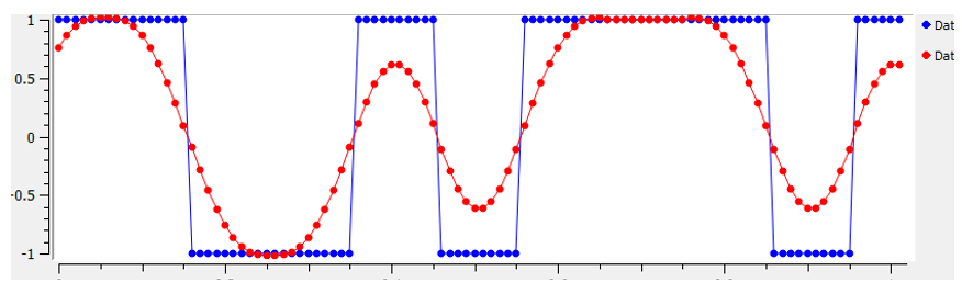
We use filters to craft the "shape" of our symbols considering the shape in the fourth dimension domain changes the shape in the frequency domain. The frequency domain informs us how much spectrum/bandwidth our signal will use, and nosotros ordinarily want to minimize it. What is of import to understand is that the spectral characteristics (frequency domain) of the baseband symbols do not change when we modulate a carrier; information technology merely shifts the baseband up in frequency while the shape stays the same, which means the corporeality of bandwidth it uses stays the same. When we use one sample per symbol, it's like transmitting square pulses. In fact BPSK using 1 sample per symbol is just a foursquare wave of random 1'southward and -1's:

And every bit we accept learned, square pulses are not efficient considering they utilize an excess amount of spectrum:

So what we do is we "pulse shape" these blocky-looking symbols so that they accept up less bandwidth in the frequency domain. We "pulse shape" by using a low-pass filter because it discards the higher frequency components of our symbols. Below shows an example of symbols in the time (top) and frequency (bottom) domain, earlier and after a pulse-shaping filter has been practical:
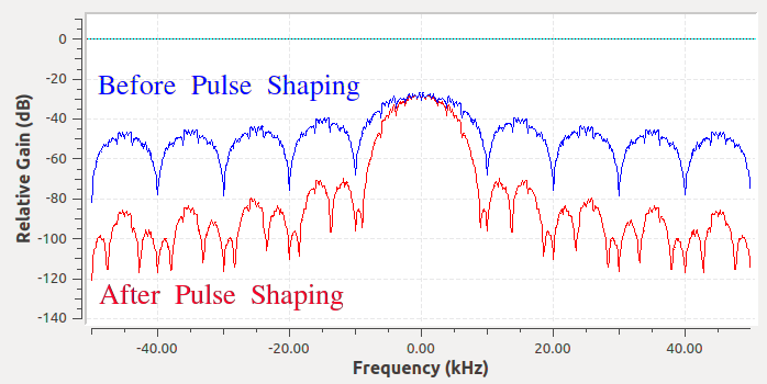
Notation how much quicker the indicate drops off in frequency. The sidelobes are ~thirty dB lower subsequently pulse shaping; that'south one,000x less! And more chiefly, the main lobe is narrower, so less spectrum is used for the same amount of $.25 per 2nd.
For now, be aware that mutual pulse-shaping filters include:
- Raised-cosine filter
- Root raised-cosine filter
- Sinc filter
- Gaussian filter
These filters generally take a parameter you can adjust to decrease the bandwidth used. Beneath demonstrates the fourth dimension and frequency domain of a raised-cosine filter with unlike values of  , the parameter that defines how steep the roll-off is.
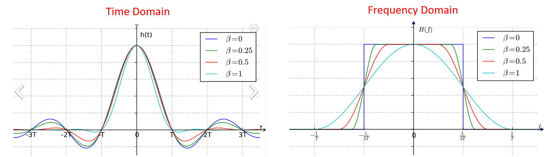
You tin can see that a lower value of reduces the spectrum used (for the same amount of information). However, if the value is also low then the fourth dimension domain symbols take longer to decay to nil. Actually when  the symbols never fully disuse to goose egg, which means we can't transmit such symbols in do. A value effectually 0.35 is common.
You will learn a lot more about pulse shaping, including some special properties that pulse shaping filters must satisfy, in the Pulse Shaping chapter.

How Many Discrete Band Pass Filters Does The 7300 Include?,
Source: https://pysdr.org/content/filters.html
Posted by: smithbutch1974.blogspot.com
0 Response to "How Many Discrete Band Pass Filters Does The 7300 Include?"
Post a Comment